library(downloadthis)
  library(dplyr)
  library(ggplot2)
  library(tidyr)
  events = c("M1", "M2", "W1", "W2")

Setup

Calculate the conditional probabilities

tbl_predictions = purrr::map_dfr(
      events,
      # read in the predictions for each event
      ~readr::read_csv(
          here::here("analyses", paste0("2024-02-16_Pem-", .x, ".csv")),
          col_types = readr::cols(
              Competitor = readr::col_character(),
              .default = readr::col_double()
          ),
      ) |>
      rename(crew_name = Competitor) |>
      # pivot to long format for easier manipulation
      pivot_longer(
          cols = !c(crew_name),
          names_to = "round",
          values_to = "prob"
      ),
      .id = "event"
  ) |>
      mutate(round = as.integer(round)) |>
      # remove mistakes in output and byes
      filter(round < 4, prob < 1)

tbl_cond_probs = tbl_predictions |>
      # calculate the conditional probability
      # p(win round A | compete in round A) = p(win round A) / p(compete in round A)
      # NB: p(compete in round A) = 1 for the first round
      group_by(crew_name) |>
      arrange(round, .by_group = TRUE) |>
      mutate(
          # probability 0 breaks things, make it up to
          # Monte Carlo error
          prob = pmax(prob, 1/1000),
          cond_prob = prob / c(lead(prob)[-n()], 1),
      ) |>
      ungroup() |>
      assertr::assert(assertr::not_na, cond_prob)
  
  tbl_cond_probs |>
      DT::datatable()

Read the results

# results contain the round each crew lost, or 0 if they won the event
  tbl_results = readr::read_csv(
      here::here("data/results/pem_regatta.csv"),
      col_types = readr::cols(
          crew_name = readr::col_character(),
          round = readr::col_integer(),
      )
  ) |>
      rename(last_round = round)
  
  tbl_results |>
      DT::datatable()

Join tables

tbl_probs_outcomes = left_join(
      tbl_cond_probs,
      tbl_results,
      by = "crew_name"
  ) |>
      filter(
          round >= last_round - 1,
          # exclude match-ups due to LMBC scratching
          crew_name != "Girton W1",
          !(crew_name == "Caius W1" & round == 3),
      ) |>
      # set outcome to 1 if the crew progressed past the round,
      # 0 if they didn't
      mutate(
          outcome = (round >= last_round),
          brier = (cond_prob - outcome)^2
      )

Should be a true and false pair for each race, hence overall 50% of outcomes are true:

tbl_probs_outcomes |>
      summarise(
          mean(outcome),
          .by = event
      )

## # A tibble: 4 × 2
  ##   event `mean(outcome)`
  ##   <chr>           <dbl>
  ## 1 4                 0.5
  ## 2 1                 0.5
  ## 3 3                 0.5
  ## 4 2                 0.5

Calibration

tbl_probs_outcomes |>
      # bin into five equal size bins based on the conditional probability
      # then check the calibration of the bins
      mutate(bin = ntile(cond_prob, 5)) |>
      summarise(
          .by = bin,
          x = sum(outcome),
          n = n(),
          mean_pred = mean(cond_prob),
      ) |>
      # exact 80% confidence intervals for binomial proportions
      mutate(
          binom::binom.confint(
              x, n,
              conf.level = 0.8,
              methods = "exact"
          )
      ) |>
      # plot with binomial confidence intervals
      ggplot(aes(x = mean_pred, y = mean)) +
      geom_point() +
      geom_errorbar(
          aes(ymin = lower,
              ymax = upper),
          width = 0
      ) +
      geom_abline(intercept = 0, slope = 1, linetype = "dashed") +
      scale_x_continuous(labels = scales::percent, limits = c(0, 1)) +
      scale_y_continuous(labels = scales::percent, limits = c(0, 1)) +
      labs(
          x = "Predicted probability",
          y = "Observed probability",
          title = "Calibration of predicted probabilities",
          subtitle = "Points are the mean observed probability in each bin, with 80% confidence intervals"
      ) +
      theme_minimal()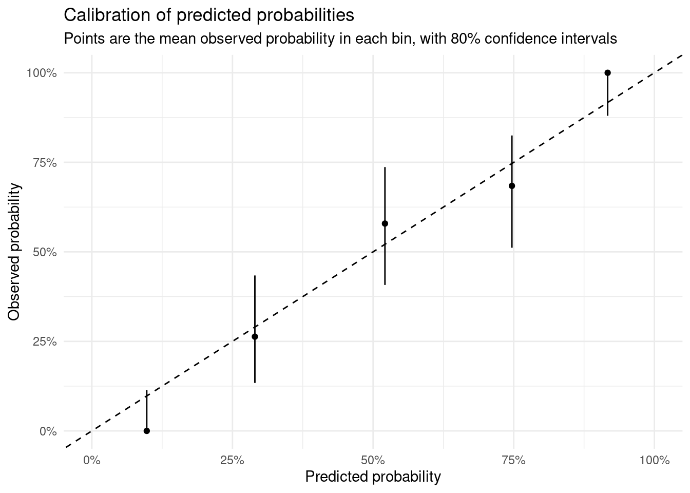

Surprising results

Mean brier score is 0.1357385 with a standard deviation of 0.1683743.

tbl_probs_outcomes |>
      ggplot(aes(brier)) +
      geom_histogram(bins = 20) +
      labs(
          x = "Brier score",
          y = "Count",
          title = "Distribution of Brier scores"
      ) +
      theme_minimal()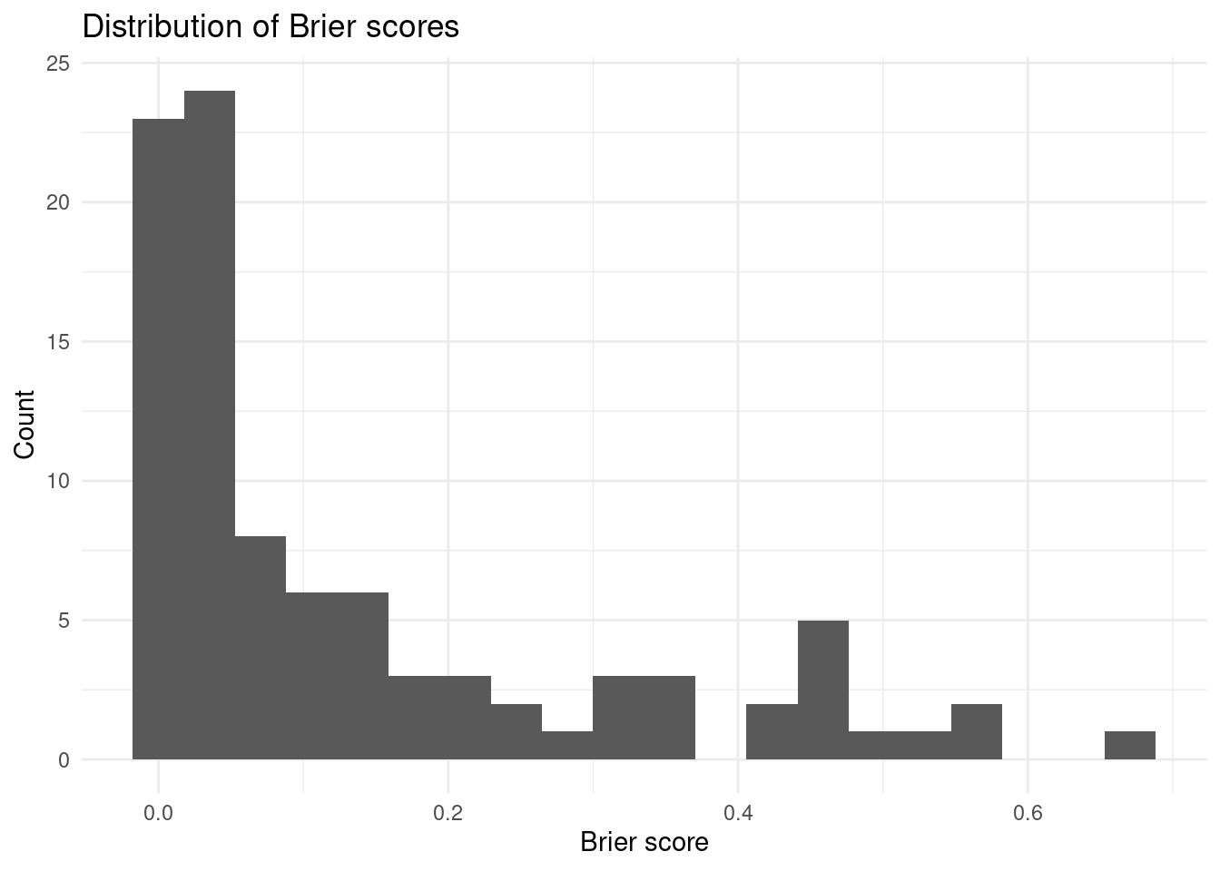

The table below shows the most surprising results, based on the brier score.

tbl_probs_outcomes |>
      # calculate the log odds of the conditional probability
      arrange(desc(brier)) |>
      DT::datatable()

Top 10 are a bit above the rest on how surprising. These matchups were (with winner bolded, grouped by event).

Clare W1 v Catz W1
Catz W1 v Emma W1
Corpus W1 v Jesus W2
Emma W2 v Hughes W1
Clare W2 v Maggie W2
Wolfson M1 v Corpus M1

Why did we underestimate Catz? Lets compare their race results to Clare and Emma.

fit_prev = readRDS(here::here("outputs/fit_archive/fit_2024-02-16_1331.rds"))
  tbl_data = tar_read(all_data)
  tbl_adjustment = fit_prev |> 
    tidybayes::spread_draws(`r_event:div`[event_div,], `b_releveleventrefEQnewnham_head(.+)`, regex = T) |> 
    mutate("b_releveleventrefEQnewnham_headnewnham_head" = 0) |> 
    pivot_longer(
      starts_with("b_releveleventrefEQnewnham_head"),
      names_prefix = "b_releveleventrefEQnewnham_head",
      values_to = "event_adjust",
      names_to = "event_adjust_event"
    ) |> 
    tidyr::extract(event_div, c("event", "div"), "^(.+)_([0-9]+)$") |> 
    filter(event == event_adjust_event) |> 
    replace_na(list(event_adjust = 0)) |> 
    group_by(event, div) |> 
    summarise(
      adjust_div = mean(`r_event:div`),
      adjust_all = mean(`r_event:div` + event_adjust)
    )

## `summarise()` has grouped output by 'event'. You can override using the
  ## `.groups` argument.

tbl_data |> 
    add_crew_name() |> 
    filter(crew_name %in% c("St. Catherine's W1", "Clare W1", "Emmanuel W1")) |>
    filter(censor == "none") |> 
    inner_join(tbl_adjustment, by = c("event", "div")) |>
    mutate(div = as.integer(div)) |>
    transmute(
      event,
      div,
      crew_name,
      raw_time = time,
      raw_split = 500 / speed,
      adjust_div_time = distance / exp(log(speed) - adjust_div),
      adjust_all_split = 500 / exp(log(speed) - adjust_all),
    ) |> 
    arrange(event, adjust_all_split) |> 
    mutate(across(c(raw_time, raw_split, adjust_div_time, adjust_all_split), display_duration)) |> 
    DT::datatable()

So Catz did pretty poorly in Head to Head. They were faster at Fairbairns, but we downweight that, and Newnham Head, but were in a fast division.